Solving a simple 2-period Consumption problem with RcppGSL
In this example we demonstrate how to solve the following problem using the RcppGSL package. GSL is the GNU scientific library and has many useful functions written in C++. RcppGSL is the Rcpp interface for R. Please look at the separate chapter "how to install RcppGSL" as that needs a trick or two.
problem
\[ \begin{array}{ccc} max_x &\log(a - x) + \beta log(x) \\ &x \in [0.1,11],\\ &a \in {2,3,\dots,10} \end{array}\]
We have a two-period problem of a consumer who has a cake of size $ a $ and needs to decide how much to consume today and how much to leave for tomorrow. The choice of how much to save, $ x $ , is a continuous variable; The size of the cake today is continuous as well, but we measure it only a set of discrete points. If we are interested at the value of having a cake size of, say, $ a = 2.7 $, we can use an interpolation technique to compute this value.
This is very simple problem. To add at least some realism, we will linearly interpolate the "future value" $ log(x) $. This should mimic a more realistic situation when our model does not admit a closed form of this object.
Solution
The good thing is that there is an analytic solution to this. Taking the derivative w.r.t. x one obtains
\[ \begin{array}{cccc} \frac{1}{a-x} &=& \beta \frac{1}{x} \\ \beta (a-x) &=& x \\ \beta a &=& x (1+\beta) \\ a\frac{\beta}{1+\beta} &=& x \end{array} \]
which implies that savings \(x\) are a constant fraction of current assets.
We will use 2 approaches to solve this problem:
- directly optimize the objective function
- solve for a root of the first order condition
Approach 1: Maximize the objective function
In this approach we want to choose \(x\) to directly maximize $ (a - x) + log(x) $ .
library(RcppGSL)## Loading required package: Rcpplibrary(inline)## Loading required package: methods
# define asset and savings grid
a <- seq(2, 10, le = 9)
x <- seq(0.1, 11, le = 50)

Beta <- 0.95
verbose <- FALSE  # set FALSE to supress printing the trace of the optimizer
Rcpp Inline
We will use the inline package to write C source code inline. Then we compile the source in place to a C function, and we call it from R. See chapter "intro to Rcpp".
GSL
It is useful to get familiar with the funcionality of the GSL library first. Please have a look around the manual of GSL relating to one-dimensional minization. In particular the setting up of the various objects can be a bit confusing initially. We are basically presenting a modified version of the example shown on that page.
RcppGSL
First, define a string "inc" to be our personal header file for the C function:
inc <- '
#include <gsl/gsl_min.h>
#include <gsl/gsl_interp.h>

// this struct will hold parameters we need in the objective
// those contain also the approximation object "myint" and
// corresponding accelerator acc
struct my_f_params { double a; double beta; const gsl_interp *myint; gsl_interp_accel *acc; NumericVector xx;NumericVector y;};

// note that we want to MAXIMIZE value, but the algorithm
// minimizes a function. we multiply return values with -1 to fix that.

double my_obj( double x, void *p){

    // define the parameter struct
    struct my_f_params *params = (struct my_f_params *)p;
    double a                   = (params->a);
    double beta                = (params->beta);
    const gsl_interp *myint    = (params->myint);
    gsl_interp_accel *acc      = (params->acc);
    NumericVector xx           = (params->xx);
    NumericVector y            = (params->y);

    double res, out, ev;

    // obtain interpolated value

    ev = gsl_interp_eval(myint, xx.begin(), y.begin(), x,acc);

    res = a - x;    //current resources

    // if consumption negative, very large penalty value
    if (res<0) {
        out =  1e9;
    } else {
        out = - (log(res) + beta*ev);
    }
    return out;
}
'
testing the objective function
It's very important to always check the objective function. here's a code snippet that will print the value of the objective at different asset and savings states:
src <- '
NumericVector a(a_); // a has the same memory address as a_
NumericVector x(x_);
double beta = as<double>(beta_);
NumericVector ay = log(x); // future values
int m = x.length();
int n = a.length();
// R is the matrix of return values
NumericMatrix R(n,m);
//initiate gsl interpolation object
gsl_interp_accel *accP = gsl_interp_accel_alloc() ;
gsl_interp *linP = gsl_interp_alloc( gsl_interp_linear , m );
gsl_interp_init( linP, x.begin(), ay.begin(), m );
// initiate a struct with params
struct my_f_params params = {a(0),beta,linP,accP,x,ay};
// initiate the gsl objective function
gsl_function F;
//point to our objective function
F.function = &my_obj;
// point my_f_params struct "params" to F
F.params = ¶ms;
// --------------------------------
// loop over rows of R: values of a
// --------------------------------
for (int i=0;i < a.length(); i++){
// notice that the value of the state a(i) changes
params.a = a(i);
// uncomment those lines to print intermediate values
//Rcout << "asset state :" << i << std::endl;
//Rcout << "asset value :" << a(i) << std::endl;
// --------------------------------
// loop over cols of R: values of x
// --------------------------------
for (int j=0; j < m; j++) {
//Rcout << "saving value :" << x(j) << std::endl;
//Rcout << GSL_FN_EVAL(&F,x(j)) << std::endl;
R(i,j) = GSL_FN_EVAL(&F,x(j));
}
}
return wrap(R);
'
# here we compile the c function:
testf=cxxfunction(signature(a_="numeric",x_="numeric",beta_="numeric"),body=src,plugin="RcppGSL",includes=inc)
# here we call it
res1 <- testf(a_=a,x_=x,beta_=Beta)
res1[res1==1e9] = NA # the value 1e9 stands for "not feasible"
persp(res1,theta=100,main="objective function",ticktype="detailed",x=a,y=x,zlab="objective function value")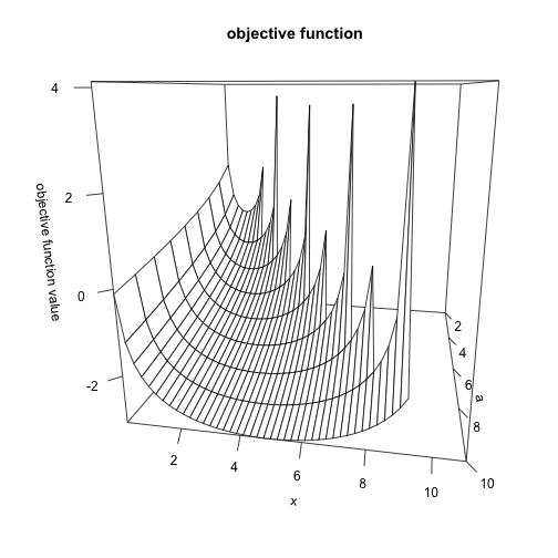
plot of chunk unnamed-chunk-3
Setup the optimizer
Now that we are more or less convinced that the objective returns sensible values, we can setup the optimizer. In terms of the above picture, for every value of a on the right axis, we want to pick different values of x and find the one that makes the objective function smallest.
src2 <- '
// map values from R
NumericVector a(a_);
NumericVector x(x_);
double beta = as<double>(beta_);
bool verbose = as<bool>(verbose_);
NumericVector ay = log(x); // future values
int na = a.length();
NumericVector R(na); // allocate a return vector
// optimizer setup
int status;
int iter=0,max_iter=100;
const gsl_min_fminimizer_type *T;
gsl_min_fminimizer *s;
int k = x.length();
gsl_interp_accel *accP = gsl_interp_accel_alloc() ;
gsl_interp *linP = gsl_interp_alloc( gsl_interp_linear , k );
gsl_interp_init( linP, x.begin(), ay.begin(), k );
// parameter struct
struct my_f_params params = {a(0),beta,linP,accP,x,ay};
// gsl objective function
gsl_function F;
F.function = &my_obj;
F.params = ¶ms;
// bounds on choice variable
double low = x(0), up=x(k-1);
double m = 0.2; //current minium
// create an fminimizer object of type "brent"
T = gsl_min_fminimizer_brent;
s = gsl_min_fminimizer_alloc(T);
printf("using %s method\\n",
gsl_min_fminimizer_name(s));
for (int i=0;i < a.length(); i++){
// load current grid values into struct
// if interpolation schemes depend on current state
// i, need to allocate linP(i) here and then load into
// params
// notice that the value of the state a(i) changes
params.a = a(i);
// if optimization bounds change do that here
low = x(0);
up=x(k-1);
iter=0; // reset iterator for each state
m = 0.2; // reset minimum for each state
// set minimzer on current obj function
gsl_min_fminimizer_set( s, &F, m, low, up );
// print results
if (verbose){
printf (" iter lower upper minimum int.length\\n");
printf ("%5d [%.7f, %.7f] %.7f %.7f\\n",
iter, low, up,m, up - low);
}
// optimization loop
do {
iter++;
status = gsl_min_fminimizer_iterate(s);
m = gsl_min_fminimizer_x_minimum(s);
low = gsl_min_fminimizer_x_lower(s);
up = gsl_min_fminimizer_x_upper(s);
status = gsl_min_test_interval(low,up,0.001,0.0);
if (status == GSL_SUCCESS && verbose){
Rprintf("Converged:\\n");
}
if (verbose){
printf ("%5d [%.7f, %.7f] %.7f %.7f\\n",
iter, low, up,m, up - low);
}
}
while (status == GSL_CONTINUE && iter < max_iter);
R(i) = m;
}
gsl_min_fminimizer_free(s);
return wrap(R);
'compiling the C function
f2=cxxfunction(signature(a_="numeric",x_="numeric",beta_="numeric",verbose_="logical"),
               body=src2,plugin="RcppGSL",includes=inc)

# setup a wrapper to call. optional
myfun <- function(ass,sav,Beta,verbose){
  res <- f2(ass,sav,Beta,verbose)
    return(res)
}

myres <- myfun(a,x,Beta,verbose)
look at result
we can compare the analytical solution to the one we found by just plotting the optimal savings choices:
plot(a, a * Beta/(1 + Beta), col = "red")
lines(a, myres)
legend("bottomright", legend = c("true", "approx"), lty = c(1, 1), col = c("red",
    "black"))
plot of chunk unnamed-chunk-6
How far is our solution from the closed form?
print(max(a * Beta/(1 + Beta) - myres))## [1] 0.05496Approach 2: Solve for a Root of the first order condition
In this example this is a bit pointless, since as we have mentioned there is a closed form solution to the first order condition. Rememember the equation is
\[ x - \beta (a - x ) = 0 \]
We will illustrate the GSL root solver to find $ x $ which satisfies this equation. The steps to take are very similar to approach 1 above, but there are some subtle differences we have to keep in mind. We begin again with an include file, where we define the changed objective function. Notice also that the required gsl include has changed:
inc <- '
#include <gsl/gsl_roots.h>

// this struct will hold parameters we need in the objective
struct my_f_params { double a; double beta; };

double my_obj( double x, void *p){
    struct my_f_params *params = (struct my_f_params *)p;
    double a                   = (params->a);
    double beta                = (params->beta);

    double res;

    res = x - beta*(a - x);
    return res;
}

// define root solver wrapper
double find_root(gsl_root_fsolver *s, gsl_function * F, double a, double b) {
  int iter = 0, max_iter = 100 ,status;
  double r, x_lo,x_hi;

  gsl_root_fsolver_set (s, F, a, b);
  do {
    iter++;
    status = gsl_root_fsolver_iterate (s);
    r      = gsl_root_fsolver_root (s);
    x_lo   = gsl_root_fsolver_x_lower (s);
    x_hi   = gsl_root_fsolver_x_upper (s);
    status = gsl_root_test_interval (x_lo, x_hi,
                                     0, 0.001);
    // if (status == GSL_SUCCESS)
    //   printf ("Converged:\\n");
    //
    // printf ("%5d [%.7f, %.7f] %.7f %+.7f %.7f\\n",
    //         iter, x_lo, x_hi,
    //         r, r - r_expected,
    //         x_hi - x_lo);
  } while (status == GSL_CONTINUE && iter < max_iter);

  return( (x_lo + x_hi)/2.0);
}
'
Objective Function Test 2
We again test our objective function.
src <- '
NumericVector a(a_); // a has the same memory address as a_
NumericVector x(x_);
double beta = as<double>(beta_);
int m = x.length();
int n = a.length();
// R is the matrix of return values
NumericMatrix R(n,m);
// param struct
struct my_f_params params = {a(0),beta};
// gsl objective function
gsl_function F;
//point to our objective function
F.function = &my_obj;
F.params = ¶ms;
// --------------------------------
// loop over rows of R: values of a
// --------------------------------
for (int i=0;i < a.length(); i++){
// define the struct on that state:
// notice that the value of the state a(i) changes
params.a = a(i);
// uncomment those lines to print intermediate values
//Rcout << "asset state :" << i << std::endl;
//Rcout << "asset value :" << a(i) << std::endl;
// --------------------------------
// loop over cols of R: values of x
// --------------------------------
for (int j=0; j < m; j++) {
//Rcout << "saving value :" << x(j) << std::endl;
//Rcout << GSL_FN_EVAL(&F,x(j)) << std::endl;
R(i,j) = GSL_FN_EVAL(&F,x(j));
}
}
return wrap(R);
'We can make a nice plot with the rgl package. Notice that the objective (red) crosses the value of zero (the blue plane) at every state. This is important, since it tells us that at every state there exists a solution to this problem.
library(rgl)
knit_hooks$set(rgl = hook_rgl)
testf = cxxfunction(signature(a_ = "numeric", x_ = "numeric", beta_ = "numeric"),
body = src, plugin = "RcppGSL", includes = inc)
# call the test
res1 <- testf(a_ = a, x_ = x, beta_ = Beta)
open3d()## [1] 1surface3d(a, x, res1 * 0.3, color = "red", alpha = 0.8) # scaled res1
axes3d(labels = FALSE, tick = FALSE)
planes3d(a = 0, b = 0, c = -1, d = 0, color = "blue", alpha = 0.8)
view3d(theta = 0, -70)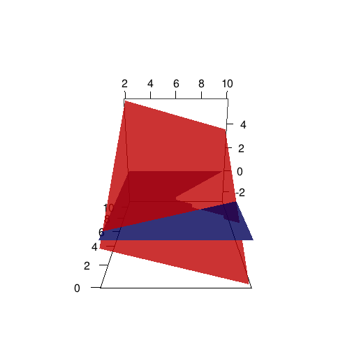
plot of chunk unnamed-chunk-11
Solve the optimization problem
src2 <- '
// map values from R
NumericVector a(a_);
NumericVector x(x_);
double beta = as<double>(beta_);
bool verbose = as<bool>(verbose_);
NumericVector ay = log(x); // future values
int na = a.length();
NumericVector R(na); // allocate a return vector
// optimizer setup
int status;
int iter=0,max_iter=100;
int k = x.length();
// initialize the root finder
const gsl_root_fsolver_type *T2 = gsl_root_fsolver_brent;
gsl_root_fsolver *rootfinder = gsl_root_fsolver_alloc (T2);
// parameter struct
struct my_f_params params = {a(0),beta};
// gsl objective function
gsl_function F;
F.function = &my_obj;
F.params = ¶ms;
// bounds on choice variable
double low = x(0), up=x(k-1);
double root;
// loop over states
for (int i=0;i < a.length(); i++){
params.a = a(i);
root = find_root( rootfinder, &F, low, up);
R(i) = root;
}
gsl_root_fsolver_free( rootfinder );
return wrap(R);
'
f2=cxxfunction(signature(a_="numeric",x_="numeric",beta_="numeric",verbose_="logical"),
body=src2,plugin="RcppGSL",includes=inc)
# setup a wrapper to call. optional
myfun <- function(ass,sav,Beta,verbose){
res <- f2(ass,sav,Beta,verbose)
return(res)
}
myres <- myfun(a,x,Beta,verbose)
#### look at result
plot(a,a*Beta/(1+Beta),col="red")
lines(a,myres)
legend("bottomright",legend=c("true","approx"),lty=c(1,1),col=c("red","black"))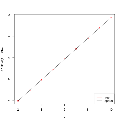
plot of chunk unnamed-chunk-12
##### How far is our solution from the closed form?

print(max(a * Beta/(1+Beta) -myres))
## [1] 4.441e-16You can see that in this instance the second approach clearly outperforms the first one. This is quite obvious, given the simple function we had to solve.