This section will describe how to use the data.table package. This package is a much faster implementation of the data.frame object which it also extends.

This is rather superficial overview of data.table where we describe briefly how to construct a panel data set with lagged variables. For a thorough overview of the capabilities of data.table, please refer to the excellent documentation of the package, for example in the vignettes at http://cran.r-project.org/web/packages/data.table/index.html

The structure of data.table

A data.table is a collection of vectors of identical length. Each vector forms a column, and so the data.table can be thought of as a table with a number of row and a number of columns.

Let's create a data.table:

require(data.table)

## Loading required package: data.table

v1 = seq(0, 1, l = 10)
v2 = sample(c("a", "b", "c"), 10, replace = TRUE)
dd = data.table(i = v1, l = v2)
dd

##          i l
##  1: 0.0000 c
##  2: 0.1111 b
##  3: 0.2222 c
##  4: 0.3333 c
##  5: 0.4444 b
##  6: 0.5556 c
##  7: 0.6667 b
##  8: 0.7778 c
##  9: 0.8889 b
## 10: 1.0000 b

Then columns can be accessed by names using the dollar sign as in a standard data.frame, or by their name, or by handling the table as a list (a data.table is a list)

# use dollar sign
dd$i

##  [1] 0.0000 0.1111 0.2222 0.3333 0.4444 0.5556 0.6667 0.7778 0.8889 1.0000

# same as using the j-argument, the list index or the the list name?
all(all.equal(dd$i,dd[,i]),
    all.equal(dd$i,dd[[1]]),
    all.equal(dd$i,dd[["i"]]))

## [1] TRUE

The 3 arguments of [ in data.table

the first argument allows to subset the data, the second allows to perform function on that subset, the third argument allows to apply the function by groups. TBD.

Using keys

Here we show how the keys optins can be used to compute lag variables in a data.table. This requires that you understood the way data.table works.

For this we are going to use a simulated dynamic panel. This panel will represent draws from an AR(1) process with a random effect

\[ y_{it} = \rho * y_{it-1} + f_{i} + u_{it} \]

Let's first generate the data in a very crude and slow way.

p = list(n = 20, t = 10, rho = 0.8, f_sd = 0.2, y0_sd = 1, u_sd = 1)

# create 1 entry per individual and draw a random length
dd = data.table(i = 1:p$n, l = rpois(p$n, p$t), y0 = rnorm(p$n, sd = p$y0_sd), 
    f = exp(rnorm(p$n, sd = p$y0_sd)))

# for each individual we create the time series
dd = dd[, {
    y = rep(0, l)
    y[1] = y0
    u = rnorm(l, sd = p$u_sd)
    for (t in 2:l) {
        y[t] = p$rho * y[t - 1] + f + u[t]
    }
    list(y = y, t = 1:l)
}, i]

we plot for a few indidividuals:

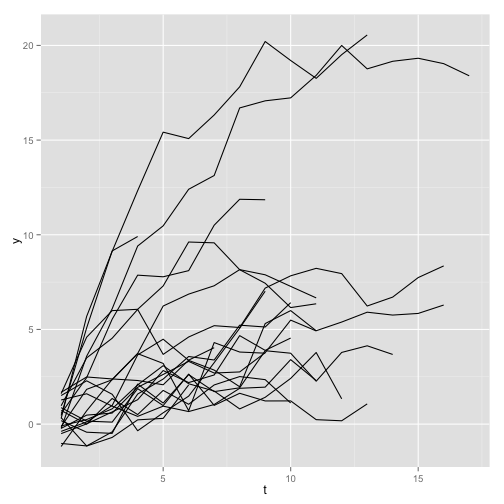
plot of chunk unnamed-chunk-4

computing panel first differences using data.table

Now that we have our data set we can create the first difference to remove the fixed effect. To do so we are going to use the keys of data.table.

We first define the keys for the table. The keys should uniquely identify a row in the data. In our case (i,t) is enough.

setkey(dd, i, t)

Next we can use the J function from the package to create the lag y

dd$y.l1 = dd[J(i, t - 1), y]$y
dd

##       i       y  t    y.l1
##   1:  1  0.3396  1      NA
##   2:  1 -1.1576  2  0.3396
##   3:  1 -0.7036  3 -1.1576
##   4:  1  0.2250  4 -0.7036
##   5:  1  0.3032  5  0.2250
##  ---                      
## 215: 20  9.5737  7  9.6171
## 216: 20  8.1554  8  9.5737
## 217: 20  7.4401  9  8.1554
## 218: 20  6.1551 10  7.4401
## 219: 20  6.3545 11  6.1551

The J function creates a data.table with the 2 columns i,j coming from the wrapping data.table. It creates a running index that will go through the table. Then we can use -1 to express that we want to shift this index by one. Any transformation can be performed at this point and one can go 4 periods before or after or anything.

Alternative approach: add lagged column by reference with :=

There is an alternative approach to the above. It differs mainly in how we add the new column containing the lagged values. When the data.table contains a lot of data, it is preferrable to manipulate it by reference, i.e. using the function :=. The following is a slight modification of a related stackoverflow.com answer. It relies on the concept of a self-join, i.e. we join the data.table to itself based on the value of a key:

setcolorder(dd,c("i","t","y","y.l1")) # change column order by reference
dd[list(i,t-1)] # evaluate at value of [lagged] key: for each i, the t index is shifted one back

##       i  t       y    y.l1
##   1:  1  0      NA      NA
##   2:  1  1  0.3396      NA
##   3:  1  2 -1.1576  0.3396
##   4:  1  3 -0.7036 -1.1576
##   5:  1  4  0.2250 -0.7036
##  ---                      
## 215: 20  6  9.6171  7.2957
## 216: 20  7  9.5737  9.6171
## 217: 20  8  8.1554  9.5737
## 218: 20  9  7.4401  8.1554
## 219: 20 10  6.1551  7.4401

dd[,y.l2 := dd[list(i,t-1)][["y"]]] # just add the "y" column of that to dd by reference

##       i  t       y    y.l1    y.l2
##   1:  1  1  0.3396      NA      NA
##   2:  1  2 -1.1576  0.3396  0.3396
##   3:  1  3 -0.7036 -1.1576 -1.1576
##   4:  1  4  0.2250 -0.7036 -0.7036
##   5:  1  5  0.3032  0.2250  0.2250
##  ---                              
## 215: 20  7  9.5737  9.6171  9.6171
## 216: 20  8  8.1554  9.5737  9.5737
## 217: 20  9  7.4401  8.1554  8.1554
## 218: 20 10  6.1551  7.4401  7.4401
## 219: 20 11  6.3545  6.1551  6.1551

dd[,all.equal(y.l1,y.l2)]

## [1] TRUE

You can see that this already produces the desired result: the value of y.